1.) Load packeges
2.) read the dat in the files, drug_coscsv, health_cos.csv in to R and assign to the variables drug_cos and health_cos, respectively
drug_cos  <- read_csv("https://estanny.com/static/week6/drug_cos.csv")
health_cos  <- read_csv("https://estanny.com/static/week6/health_cos.csv")
3.) Use glimpse to get a glimpse of the data
drug_cos %>% glimpse()
Rows: 104
Columns: 9
$ ticker       <chr> "ZTS", "ZTS", "ZTS", "ZTS", "ZTS", "ZTS", "Z...
$ name         <chr> "Zoetis Inc", "Zoetis Inc", "Zoetis Inc", "Z...
$ location     <chr> "New Jersey; U.S.A", "New Jersey; U.S.A", "N...
$ ebitdamargin <dbl> 0.149, 0.217, 0.222, 0.238, 0.182, 0.335, 0....
$ grossmargin  <dbl> 0.610, 0.640, 0.634, 0.641, 0.635, 0.659, 0....
$ netmargin    <dbl> 0.058, 0.101, 0.111, 0.122, 0.071, 0.168, 0....
$ ros          <dbl> 0.101, 0.171, 0.176, 0.195, 0.140, 0.286, 0....
$ roe          <dbl> 0.069, 0.113, 0.612, 0.465, 0.285, 0.587, 0....
$ year         <dbl> 2011, 2012, 2013, 2014, 2015, 2016, 2017, 20...
health_cos %>% glimpse()
Rows: 464
Columns: 11
$ ticker      <chr> "ZTS", "ZTS", "ZTS", "ZTS", "ZTS", "ZTS", "ZT...
$ name        <chr> "Zoetis Inc", "Zoetis Inc", "Zoetis Inc", "Zo...
$ revenue     <dbl> 4233000000, 4336000000, 4561000000, 478500000...
$ gp          <dbl> 2581000000, 2773000000, 2892000000, 306800000...
$ rnd         <dbl> 427000000, 409000000, 399000000, 396000000, 3...
$ netincome   <dbl> 245000000, 436000000, 504000000, 583000000, 3...
$ assets      <dbl> 5711000000, 6262000000, 6558000000, 658800000...
$ liabilities <dbl> 1975000000, 2221000000, 5596000000, 525100000...
$ marketcap   <dbl> NA, NA, 16345223371, 21572007994, 23860348635...
$ year        <dbl> 2011, 2012, 2013, 2014, 2015, 2016, 2017, 201...
$ industry    <chr> "Drug Manufacturers - Specialty & Generic", "...
4.) Which variables are the same in both data sets
names_drug  <- drug_cos  %>%  names()
names_health  <- health_cos  %>%  names()
intersect(names_drug, names_health)
[1] "ticker" "name" "year" 5.) Select subset of variables to work with For drug_cos select (in this order): ticker, year, grossmargin
Extract observations for 2018
Assign output to drug_subset
For health_cos select (in this order): ticker, year, revenue, gp, industry
Extract observations for 2018
Assign output to health_subset
6.) Keep all the rows and columns drug_subset join with columns in health_subset
drug_subset %>% left_join(health_subset)
# A tibble: 13 x 6
   ticker  year grossmargin   revenue        gp industry
   <chr>  <dbl>       <dbl>     <dbl>     <dbl> <chr>
 1 ZTS     2018       0.672   5.82e 9   3.91e 9 Drug Manufacturers - ~
 2 PRGO    2018       0.387   4.73e 9   1.83e 9 Drug Manufacturers - ~
 3 PFE     2018       0.79    5.36e10   4.24e10 Drug Manufacturers - ~
 4 MYL     2018       0.35    1.14e10   4.00e 9 Drug Manufacturers - ~
 5 MRK     2018       0.681   4.23e10   2.88e10 Drug Manufacturers - ~
 6 LLY     2018       0.738   2.46e10   1.81e10 Drug Manufacturers - ~
 7 JNJ     2018       0.668   8.16e10   5.45e10 Drug Manufacturers - ~
 8 GILD    2018       0.781   2.21e10   1.73e10 Drug Manufacturers - ~
 9 BMY     2018       0.71    2.26e10   1.60e10 Drug Manufacturers - ~
10 BIIB    2018       0.865   1.35e10   1.16e10 Drug Manufacturers - ~
11 AMGN    2018       0.827   2.37e10   1.96e10 Drug Manufacturers - ~
12 AGN     2018       0.861   1.58e10   1.36e10 Drug Manufacturers - ~
13 ABBV    2018       0.764   3.28e10   2.50e10 Drug Manufacturers - ~
quiz questions
Start with drug_cos
Extract observations for the ticker SEE QUIZ from drug_cos
Assign output to the variable drug_cos_subset
drug_cos_subset  <- drug_cos  %>%
  filter(ticker == "BIIB")
Display drug_cos_subset
drug_cos_subset
# A tibble: 8 x 9
  ticker name  location ebitdamargin grossmargin netmargin   ros   roe
  <chr>  <chr> <chr>           <dbl>       <dbl>     <dbl> <dbl> <dbl>
1 BIIB   Biog~ Massach~        0.404       0.908     0.245 0.333 0.204
2 BIIB   Biog~ Massach~        0.402       0.901     0.25  0.335 0.211
3 BIIB   Biog~ Massach~        0.432       0.876     0.269 0.355 0.233
4 BIIB   Biog~ Massach~        0.475       0.879     0.302 0.404 0.294
5 BIIB   Biog~ Massach~        0.493       0.885     0.33  0.437 0.321
6 BIIB   Biog~ Massach~        0.491       0.871     0.323 0.431 0.322
7 BIIB   Biog~ Massach~        0.495       0.867     0.207 0.407 0.209
8 BIIB   Biog~ Massach~        0.511       0.865     0.329 0.435 0.334
# ... with 1 more variable: year <dbl>
Use left_join to combine the rows and columns of drug_cos_subset with the columns of health_cos
Assign the output to combo_df
combo_df <- drug_cos_subset  %>%
  left_join(health_cos)
Display combo_df
combo_df
# A tibble: 8 x 17
  ticker name  location ebitdamargin grossmargin netmargin   ros   roe
  <chr>  <chr> <chr>           <dbl>       <dbl>     <dbl> <dbl> <dbl>
1 BIIB   Biog~ Massach~        0.404       0.908     0.245 0.333 0.204
2 BIIB   Biog~ Massach~        0.402       0.901     0.25  0.335 0.211
3 BIIB   Biog~ Massach~        0.432       0.876     0.269 0.355 0.233
4 BIIB   Biog~ Massach~        0.475       0.879     0.302 0.404 0.294
5 BIIB   Biog~ Massach~        0.493       0.885     0.33  0.437 0.321
6 BIIB   Biog~ Massach~        0.491       0.871     0.323 0.431 0.322
7 BIIB   Biog~ Massach~        0.495       0.867     0.207 0.407 0.209
8 BIIB   Biog~ Massach~        0.511       0.865     0.329 0.435 0.334
# ... with 9 more variables: year <dbl>, revenue <dbl>, gp <dbl>,
#   rnd <dbl>, netincome <dbl>, assets <dbl>, liabilities <dbl>,
#   marketcap <dbl>, industry <chr>
Assign the company name to co_name
co_name  <- combo_df  %>%
  distinct(name) %>%
  pull()
Assign the company location to co_location
co_location  <- combo_df  %>%
  distinct(location)  %>%
  pull()
Assign the industry to co_industry group
co_industry  <- combo_df  %>%
  distinct(name)  %>%
  pull()
Put the r inline commands used in the blanks below. When you knit the document the results of the commands will be displayed in your text.
The company ??? is located in ??? and is a member of the ??? industry group.
Start with combo_df
Select variables (in this order): year, grossmargin, netmargin, revenue, gp, netincome
Assign the output to combo_df_subset
combo_df_subset  <- combo_df  %>%
  select(year, grossmargin, netmargin,
  revenue, gp, netincome)
combo_df_subset
# A tibble: 8 x 6
   year grossmargin netmargin     revenue          gp  netincome
  <dbl>       <dbl>     <dbl>       <dbl>       <dbl>      <dbl>
1  2011       0.908     0.245  5048634000  4581854000 1234428000
2  2012       0.901     0.25   5516461000  4970967000 1380033000
3  2013       0.876     0.269  6932200000  6074500000 1862300000
4  2014       0.879     0.302  9703300000  8532300000 2934800000
5  2015       0.885     0.33  10763800000  9523400000 3547000000
6  2016       0.871     0.323 11448800000  9970100000 3702800000
7  2017       0.867     0.207 12273900000 10643900000 2539100000
8  2018       0.865     0.329 13452900000 11636600000 4430700000
Create the variable grossmargin_check to compare with the variable grossmargin. They should be equal. grossmargin_check = gp / revenue Create the variable close_enough to check that the absolute value of the difference between grossmargin_check and grossmargin is less than 0.001
combo_df_subset  %>%
  mutate(grossmargin_check = gp / revenue,
  close_enough = abs(grossmargin_check - grossmargin) < 0.001)
# A tibble: 8 x 8
   year grossmargin netmargin revenue      gp netincome
  <dbl>       <dbl>     <dbl>   <dbl>   <dbl>     <dbl>
1  2011       0.908     0.245 5.05e 9 4.58e 9    1.23e9
2  2012       0.901     0.25  5.52e 9 4.97e 9    1.38e9
3  2013       0.876     0.269 6.93e 9 6.07e 9    1.86e9
4  2014       0.879     0.302 9.70e 9 8.53e 9    2.93e9
5  2015       0.885     0.33  1.08e10 9.52e 9    3.55e9
6  2016       0.871     0.323 1.14e10 9.97e 9    3.70e9
7  2017       0.867     0.207 1.23e10 1.06e10    2.54e9
8  2018       0.865     0.329 1.35e10 1.16e10    4.43e9
# ... with 2 more variables: grossmargin_check <dbl>,
#   close_enough <lgl>
Create the variable netmargin_check to compare with the variable netmargin. They should be equal.
Create the variable close_enough to check that the absolute value of the difference between netmargin_check and netmargin is less than 0.001
combo_df_subset %>%
  mutate(netmargin_check = netincome / revenue,
  close_enough = abs(netmargin_check - netmargin) < 0.001)
# A tibble: 8 x 8
   year grossmargin netmargin revenue      gp netincome
  <dbl>       <dbl>     <dbl>   <dbl>   <dbl>     <dbl>
1  2011       0.908     0.245 5.05e 9 4.58e 9    1.23e9
2  2012       0.901     0.25  5.52e 9 4.97e 9    1.38e9
3  2013       0.876     0.269 6.93e 9 6.07e 9    1.86e9
4  2014       0.879     0.302 9.70e 9 8.53e 9    2.93e9
5  2015       0.885     0.33  1.08e10 9.52e 9    3.55e9
6  2016       0.871     0.323 1.14e10 9.97e 9    3.70e9
7  2017       0.867     0.207 1.23e10 1.06e10    2.54e9
8  2018       0.865     0.329 1.35e10 1.16e10    4.43e9
# ... with 2 more variables: netmargin_check <dbl>,
#   close_enough <lgl>
Question 3 Summarize_industry
Fill in the blanks
Put the command you use in the Rchunks in the Rmd file for this quiz
Use the health_cos data
For each industry calculate
SEE QUIZ = mean(SEE QUIZ / revenue) * 100 SEE QUIZ = median(SEE QUIZ / revenue) * 100 SEE QUIZ = min(SEE QUIZ / revenue) * 100 SEE QUIZ = max(SEE QUIZ / revenue) * 100 health_cos %>%health_cos %>%
group_by(industry) %>%
summarize(mean_netmargin_percent = mean(netincome / revenue) * 100,
median_netmargin_percent = median(netincome / revenue) * 100,
min_netmargin_percent = min(netincome / revenue) * 100,
max_netmargin_percent = max(netincome / revenue) * 100)
# A tibble: 9 x 5
  industry mean_netmargin_~ median_netmargi~ min_netmargin_p~
* <chr>               <dbl>            <dbl>            <dbl>
1 Biotech~            -4.66             7.62         -197.
2 Diagnos~            13.1             12.3             0.399
3 Drug Ma~            19.4             19.5           -34.9
4 Drug Ma~             5.88             9.01          -76.0
5 Healthc~             3.28             3.37           -0.305
6 Medical~             6.10             6.46            1.40
7 Medical~            12.4             14.3           -56.1
8 Medical~             1.70             1.03           -0.102
9 Medical~            12.3             14.0           -47.1
# ... with 1 more variable: max_netmargin_percent <dbl>
inline ticker question Fill in the blanks
Use the health_cos data
Extract observations for the ticker ZTS SEE QUIZ from health_cos and assign to the variable health_cos_subset
health_cos_subset  <- health_cos  %>%
  filter(ticker == "ZTS")
Display health_cos_subset
health_cos_subset
# A tibble: 8 x 11
  ticker name  revenue     gp    rnd netincome  assets liabilities
  <chr>  <chr>   <dbl>  <dbl>  <dbl>     <dbl>   <dbl>       <dbl>
1 ZTS    Zoet~  4.23e9 2.58e9 4.27e8    2.45e8 5.71e 9  1975000000
2 ZTS    Zoet~  4.34e9 2.77e9 4.09e8    4.36e8 6.26e 9  2221000000
3 ZTS    Zoet~  4.56e9 2.89e9 3.99e8    5.04e8 6.56e 9  5596000000
4 ZTS    Zoet~  4.78e9 3.07e9 3.96e8    5.83e8 6.59e 9  5251000000
5 ZTS    Zoet~  4.76e9 3.03e9 3.64e8    3.39e8 7.91e 9  6822000000
6 ZTS    Zoet~  4.89e9 3.22e9 3.76e8    8.21e8 7.65e 9  6150000000
7 ZTS    Zoet~  5.31e9 3.53e9 3.82e8    8.64e8 8.59e 9  6800000000
8 ZTS    Zoet~  5.82e9 3.91e9 4.32e8    1.43e9 1.08e10  8592000000
# ... with 3 more variables: marketcap <dbl>, year <dbl>,
#   industry <chr>
In the console, type ?distinct. Go to the help pane to see what distinct does In the console, type ?pull. Go to the help pane to see what pull does
Run the code below
health_cos_subset  %>%
  distinct(name) %>%
  pull(name)
[1] "Zoetis Inc"assign the output to co_name
co_name  <- health_cos_subset  %>%
  distinct(name) %>%
  pull(name)
You can take output from your code and include it in your text.
The name of the company with ticker SEE QUIZ is ________ In following chuck
Assign the company’s industry group to the variable co_industry
co_industry  <- health_cos_subset  %>%
  distinct(industry) %>%
  pull()
The company zoetis inc is a member of the Biogen inc group.
7.) Prepare the data for the plots start with health_cos THEN group_by industry THEN calculate the median research and development expenditure as a percent of revenue by industry assign the output to df
8.) Use glimpse to glimpse the data for the plots
df %>% glimpse()
Rows: 9
Columns: 2
$ industry <chr> "Biotechnology", "Diagnostics & Research", "D...
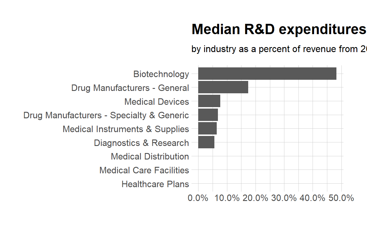
$ med_rnd_rev <dbl> 0.48317287, 0.05620271, 0.17451442, 0.0685187...9.) create a static bar chart
use ggplot to initialize the chart data is df the variable industry is mapped to the x-axis reorder it based the value of med_rnd_rev the variable med_rnd_rev is mapped to the y-axis add a bar chart using geom_col use scale_y_continuous to label the y-axis with percent use coord_flip() to flip the coordinates use labs to add title, subtitle and remove x and y-axes use theme_ipsum() from the hrbrthemes package to improve the theme
ggplot(data = df,
       mapping = aes(
         x = reorder(industry, med_rnd_rev ),
         y = med_rnd_rev
         )) +
  geom_col() +
  scale_y_continuous(labels = scales::percent) +
  coord_flip() +
  labs(
    title = "Median R&D expenditures",
    subtitle = "by industry as a percent of revenue from 2011 to 2018",
    x = NULL, y = NULL) +
  theme_ipsum()
10.) save plot to preview.png and add to the yaml chunk at the top
ggsave(filename = "preview.png",
       path = here::here("_posts", "2021-03-16-joining-data"))
11.) Create an interactive bar chart using the package echarts4r
df  %>%
  arrange(med_rnd_rev)  %>%
  e_charts(
    x = industry
    )  %>%
  e_bar(
    serie = med_rnd_rev,
    name = "median"
    )  %>%
  e_flip_coords()  %>%
  e_tooltip()  %>%
  e_title(
    text = "Median industry R&D expenditures",
    subtext = "by industry as a percent of revenue from 2011 to 2018",
    left = "center") %>%
  e_legend(FALSE) %>%
  e_x_axis(
    formatter = e_axis_formatter("percent", digits = 0)
    )  %>%
  e_y_axis(
    show = FALSE
  )  %>%
  e_theme("infographic")