Load Packages
library(tidyverse)
library(moderndive) #install before loading
library(infer) #install before loading
library(fivethirtyeight) #install before loading
library(skimr)
What is the average age of members that have served in congress?
set.seed(123)

congress_age_100 <- congress_age  %>%
  rep_sample_n(size=100)
1.) Construct the confidence interval
congress_age_100  %>%
  specify(response = age)
Response: age (numeric)
# A tibble: 100 x 1
     age
   <dbl>
 1  53.1
 2  54.9
 3  65.3
 4  60.1
 5  43.8
 6  57.9
 7  55.3
 8  46
 9  42.1
10  37
# ... with 90 more rows
calculate
function (x, stat = c("mean", "median", "sum", "sd", "prop",
    "count", "diff in means", "diff in medians", "diff in props",
    "Chisq", "F", "slope", "correlation", "t", "z", "ratio of props",
    "odds ratio"), order = NULL, ...)
{
    check_type(x, tibble::is_tibble)
    check_type(stat, rlang::is_string)
    check_for_numeric_stat(x, stat)
    check_for_factor_stat(x, stat, explanatory_variable(x))
    check_args_and_attr(x, explanatory_variable(x), response_variable(x),
        stat)
    check_point_params(x, stat)
    if (!has_response(x)) {
        stop_glue("The response variable is not set. Make sure to `specify()` it first.")
    }
    if (is_nuat(x, "generate") || !attr(x, "generate")) {
        if (!is_hypothesized(x)) {
            x$replicate <- 1L
        }
        else if (stat %in% c("mean", "median", "sum", "sd", "prop",
            "count", "diff in means", "diff in medians", "diff in props",
            "slope", "correlation", "ratio of props", "odds ratio")) {
            stop_glue("Theoretical distributions do not exist (or have not been ",
                "implemented) for `stat` = \"{stat}\". Are you missing ",
                "a `generate()` step?")
        }
        else if (!(stat %in% c("Chisq", "prop", "count")) & !(stat %in%
            c("t", "z") & (attr(x, "theory_type") %in% c("One sample t",
            "One sample prop z", "Two sample props z")))) {
            return(x)
        }
    }
    if ((stat %in% c("diff in means", "diff in medians", "diff in props",
        "ratio of props", "odds ratio")) || (!is_nuat(x, "theory_type") &&
        (attr(x, "theory_type") %in% c("Two sample props z",
            "Two sample t")))) {
        order <- check_order(x, explanatory_variable(x), order)
    }
    if (!((stat %in% c("diff in means", "diff in medians", "diff in props",
        "ratio of props", "odds ratio")) || (!is_nuat(x, "theory_type") &&
        attr(x, "theory_type") %in% c("Two sample props z", "Two sample t")))) {
        if (!is.null(order)) {
            warning_glue("Statistic is not based on a difference or ratio; the `order` argument",
                " will be ignored. Check `?calculate` for details.")
        }
    }
    result <- calc_impl(structure(stat, class = gsub(" ", "_",
        stat)), x, order, ...)
    if ("NULL" %in% class(result)) {
        stop_glue("Your choice of `stat` is invalid for the types of variables `specify`ed.")
    }
    result <- copy_attrs(to = result, from = x)
    attr(result, "stat") <- stat
    if (nrow(result) == 1) {
        result <- select(result, stat)
    }
    result
}
<bytecode: 0x000000001931f4d8>
<environment: namespace:infer>
2.) generate 1000 replicates of your sample of 100
Response: age (numeric)
# A tibble: 100,000 x 2
# Groups:   replicate [1,000]
   replicate   age
       <int> <dbl>
 1         1  42.1
 2         1  71.2
 3         1  45.6
 4         1  39.6
 5         1  56.8
 6         1  71.6
 7         1  60.5
 8         1  56.4
 9         1  43.3
10         1  53.1
# ... with 99,990 more rows
3.) calculate the mean for each replicate
bootstrap_distribution_mean_age  <- congress_age_100  %>%
  specify(response = age)  %>%
  generate(reps = 1000, type = "bootstrap")  %>%
  calculate(stat = "mean")
bootstrap_distribution_mean_age
# A tibble: 1,000 x 2
replicate stat
* <int> <dbl>
1 1 53.6
2 2 53.2
3 3 52.8
4 4 51.5
5 5 53.0
6 6 54.2
7 7 52.0
8 8 52.8
9 9 53.8
10 10 52.4
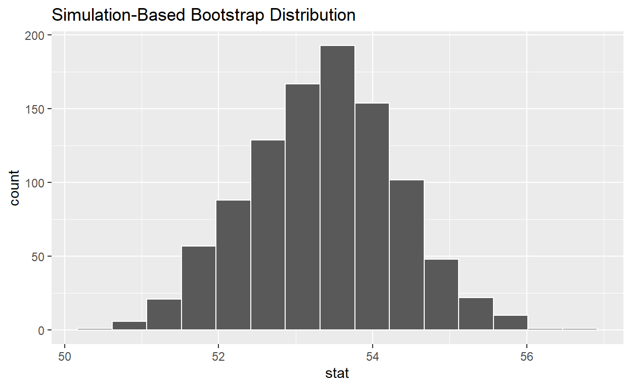
# ... with 990 more rows4.) visualize the bootstrap distribution
visualize(bootstrap_distribution_mean_age)
Calculate the 95% confidence interval using the percentile method
congress_ci_percentile  <- bootstrap_distribution_mean_age %>%
  get_confidence_interval(type = "percentile", level = 0.95)

congress_ci_percentile
# A tibble: 1 x 2
  lower_ci upper_ci
     <dbl>    <dbl>
1     51.5     55.2
Calculate the observed point estimate of the mean and assign it to obs_mean_age
obs_mean_age  <- congress_age_100    %>%
  specify(response = age)  %>%
  calculate(stat = "mean")  %>%
  pull()

obs_mean_age
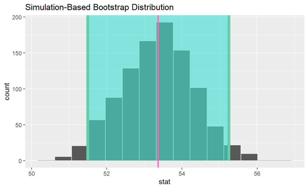
[1] 53.36shade confidence interval
visualize(bootstrap_distribution_mean_age) +
  shade_confidence_interval(endpoints = congress_ci_percentile ) +
  geom_vline(xintercept = obs_mean_age, color = "hotpink", size = 1 )
Calculate the population mean to see if it is in the 95% confidence interval
Assign the output to pop_mean_age
Display pop_mean_age
pop_mean_age  <-  congress_age_100    %>%
  summarize(pop_mean= mean(age))  %>% pull()
pop_mean_age
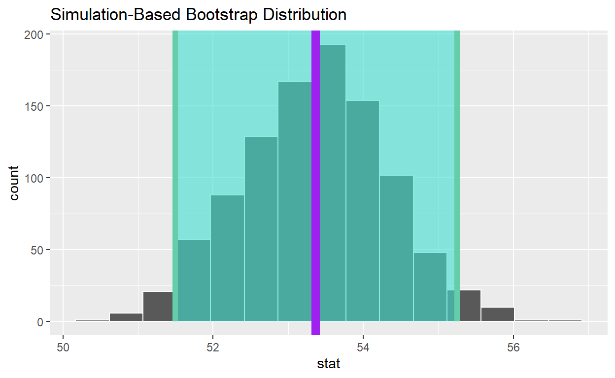
[1] 53.36Add a line to the visualization at the, population mean, pop_mean_age, to the plot color it “purple”
visualize(bootstrap_distribution_mean_age) +
  shade_confidence_interval(endpoints = congress_ci_percentile) +
   geom_vline(xintercept = obs_mean_age, color = "hotpink", size = 1) +
   geom_vline(xintercept = pop_mean_age , color = "purple", size = 3)
hr  <- read_csv("https://estanny.com/static/week13/data/hr_3_tidy.csv",
                col_types = "fddfff")
skim(hr)
| Name | hr |
| Number of rows | 500 |
| Number of columns | 6 |
| _______________________ | |
| Column type frequency: | |
| factor | 4 |
| numeric | 2 |
| ________________________ | |
| Group variables | None |
Variable type: factor
| skim_variable | n_missing | complete_rate | ordered | n_unique | top_counts |
|---|---|---|---|---|---|
| gender | 0 | 1 | FALSE | 2 | fem: 253, mal: 247 |
| evaluation | 0 | 1 | FALSE | 4 | bad: 148, fai: 138, goo: 122, ver: 92 |
| salary | 0 | 1 | FALSE | 6 | lev: 98, lev: 87, lev: 87, lev: 86 |
| status | 0 | 1 | FALSE | 3 | fir: 196, pro: 172, ok: 132 |
Variable type: numeric
| skim_variable | n_missing | complete_rate | mean | sd | p0 | p25 | p50 | p75 | p100 | hist |
|---|---|---|---|---|---|---|---|---|---|---|
| age | 0 | 1 | 39.41 | 11.33 | 20 | 29.9 | 39.35 | 49.1 | 59.9 | ▇▇▇▇▆ |
| hours | 0 | 1 | 49.68 | 13.24 | 35 | 38.2 | 45.50 | 58.8 | 79.9 | ▇▃▃▂▂ |
null_t_distribution <- hr  %>%
  specify(response = age)  %>%
  hypothesize(null = "point", mu = 48)  %>%
  generate(reps = 1000, type = "bootstrap")  %>%
  calculate(stat = "mean")
null_t_distribution
# A tibble: 1,000 x 2
   replicate  stat
 *     <int> <dbl>
 1         1  47.9
 2         2  49.4
 3         3  48.7
 4         4  48.1
 5         5  47.2
 6         6  47.9
 7         7  47.7
 8         8  47.4
 9         9  47.4
10        10  48.4
# ... with 990 more rowshr_2 <- read_csv("https://estanny.com/static/week13/data/hr_3_tidy.csv", col_types = "fddfff")
hr_2 %>%
  group_by(gender) %>%
  skim()
| Name | Piped data |
| Number of rows | 500 |
| Number of columns | 6 |
| _______________________ | |
| Column type frequency: | |
| factor | 3 |
| numeric | 2 |
| ________________________ | |
| Group variables | gender |
Variable type: factor
| skim_variable | gender | n_missing | complete_rate | ordered | n_unique | top_counts |
|---|---|---|---|---|---|---|
| evaluation | male | 0 | 1 | FALSE | 4 | bad: 72, fai: 67, goo: 61, ver: 47 |
| evaluation | female | 0 | 1 | FALSE | 4 | bad: 76, fai: 71, goo: 61, ver: 45 |
| salary | male | 0 | 1 | FALSE | 6 | lev: 47, lev: 43, lev: 43, lev: 42 |
| salary | female | 0 | 1 | FALSE | 6 | lev: 51, lev: 46, lev: 45, lev: 43 |
| status | male | 0 | 1 | FALSE | 3 | fir: 98, pro: 81, ok: 68 |
| status | female | 0 | 1 | FALSE | 3 | fir: 98, pro: 91, ok: 64 |
Variable type: numeric
| skim_variable | gender | n_missing | complete_rate | mean | sd | p0 | p25 | p50 | p75 | p100 | hist |
|---|---|---|---|---|---|---|---|---|---|---|---|
| age | male | 0 | 1 | 38.23 | 10.86 | 20 | 28.9 | 37.9 | 47.05 | 59.9 | ▇▇▇▇▅ |
| age | female | 0 | 1 | 40.56 | 11.67 | 20 | 31.0 | 40.3 | 50.50 | 59.8 | ▆▆▇▆▇ |
| hours | male | 0 | 1 | 49.55 | 13.11 | 35 | 38.4 | 45.4 | 57.65 | 79.9 | ▇▃▂▂▂ |
| hours | female | 0 | 1 | 49.80 | 13.38 | 35 | 38.2 | 45.6 | 59.40 | 79.8 | ▇▂▃▂▂ |
hr_2 %>%
  specify(response = hours, explanatory = gender)  %>%
  hypothesize(null = "independence")  %>%
  generate(reps=1000,type= "permute")
Response: hours (numeric)
Explanatory: gender (factor)
Null Hypothesis: independence
# A tibble: 500,000 x 3
# Groups:   replicate [1,000]
   hours gender replicate
   <dbl> <fct>      <int>
 1  59.9 male           1
 2  37   female         1
 3  38.9 female         1
 4  36.4 male           1
 5  58.7 male           1
 6  35   female         1
 7  38.4 female         1
 8  70.6 female         1
 9  38.9 female         1
10  57   male           1
# ... with 499,990 more rows