SEE QUIZ is the name of your data subset
Read it into and assign to hr
Note: col_types = “fddfff” defines the column types factor-double-double-factor-factor-factor
hr  <- read_csv("https://estanny.com/static/week13/data/hr_3_tidy.csv",
                col_types = "fddfff")
use the skim to summarize the data in hr
skim(hr)
| Name | hr |
| Number of rows | 500 |
| Number of columns | 6 |
| _______________________ | |
| Column type frequency: | |
| factor | 4 |
| numeric | 2 |
| ________________________ | |
| Group variables | None |
Variable type: factor
| skim_variable | n_missing | complete_rate | ordered | n_unique | top_counts |
|---|---|---|---|---|---|
| gender | 0 | 1 | FALSE | 2 | fem: 253, mal: 247 |
| evaluation | 0 | 1 | FALSE | 4 | bad: 148, fai: 138, goo: 122, ver: 92 |
| salary | 0 | 1 | FALSE | 6 | lev: 98, lev: 87, lev: 87, lev: 86 |
| status | 0 | 1 | FALSE | 3 | fir: 196, pro: 172, ok: 132 |
Variable type: numeric
| skim_variable | n_missing | complete_rate | mean | sd | p0 | p25 | p50 | p75 | p100 | hist |
|---|---|---|---|---|---|---|---|---|---|---|
| age | 0 | 1 | 39.41 | 11.33 | 20 | 29.9 | 39.35 | 49.1 | 59.9 | ▇▇▇▇▆ |
| hours | 0 | 1 | 49.68 | 13.24 | 35 | 38.2 | 45.50 | 58.8 | 79.9 | ▇▃▃▂▂ |
The mean hours worked per week is: 49.7
Q: Is the mean number of hours worked per week 48? specify that hours is the variable of interesthr %>%
specify(response = hours)
Response: hours (numeric)
# A tibble: 500 x 1
hours
<dbl>
1 49.6
2 39.2
3 63.2
4 42.2
5 54.7
6 54.3
7 37.3
8 45.6
9 35.1
10 53
# ... with 490 more rowshypothesize that the average hours worked is 48
hr  %>%
specify(response = hours) %>%
hypothesise(null = "point", mu = 48)
Response: hours (numeric)
Null Hypothesis: point
# A tibble: 500 x 1
   hours
   <dbl>
 1  49.6
 2  39.2
 3  63.2
 4  42.2
 5  54.7
 6  54.3
 7  37.3
 8  45.6
 9  35.1
10  53
# ... with 490 more rows
generate 1000 replicates representing the null hypothesis
hr %>%
  specify(response = hours)  %>%
  hypothesize(null = "point", mu = 48)  %>%
  generate(reps = 1000, type = "bootstrap")
Response: hours (numeric)
Null Hypothesis: point
# A tibble: 500,000 x 2
# Groups:   replicate [1,000]
   replicate hours
       <int> <dbl>
 1         1  40.8
 2         1  33.4
 3         1  54.6
 4         1  51.5
 5         1  33.3
 6         1  44.6
 7         1  34.1
 8         1  47.0
 9         1  34.2
10         1  55.1
# ... with 499,990 more rows
The output has 500000 rows
calculate the distribution of statistics from the generated data
Assign the output null_t_distribution
Display null_t_distribution
null_t_distribution <- hr  %>%
  specify(response = age)  %>%
  hypothesize(null = "point", mu = 48)  %>%
  generate(reps = 1000, type = "bootstrap")  %>%
  calculate(stat = "mean")
null_t_distribution
# A tibble: 1,000 x 2
replicate stat
* <int> <dbl>
1 1 47.3
2 2 47.3
3 3 48.7
4 4 47.9
5 5 47.9
6 6 47.5
7 7 47.7
8 8 48.0
9 9 48.2
10 10 48.2
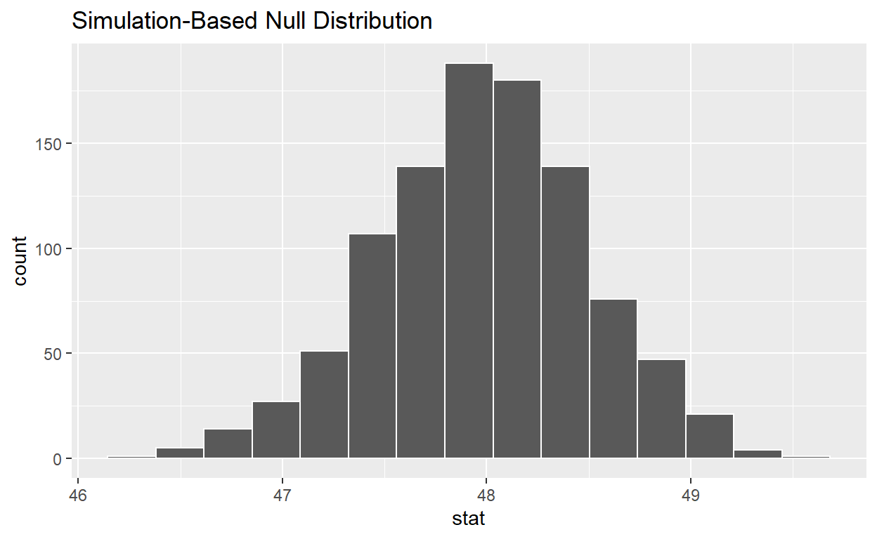
# ... with 990 more rowsnull_t_distribution has 10 t-stats
visualise(null_t_distribution)
calculate the statistic from your observed data
Assign the output observed_t_statistic
Display observed_t_statistic
observed_t_statistic  <- hr  %>%
  specify(response = hours)  %>%
  hypothesize(null = "point", mu = 48)  %>%
  calculate(stat = "t")
observed_t_statistic
# A tibble: 1 x 1
   stat
  <dbl>
1  2.83
get_p_value from the simulated null distribution and the observed statistic
null_t_distribution  %>%
  get_p_value(obs_stat = observed_t_statistic , direction = "two-sided")
# A tibble: 1 x 1
p_value
<dbl>
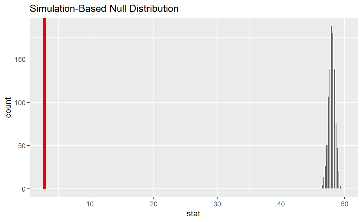
1 0shade_p_value on the simulated null distribution
null_t_distribution  %>%
  visualize() +
  shade_p_value(obs_stat = observed_t_statistic, direction = "two-sided")
Question 2
SEE QUIZ is the name of your data subset
Read it into and assign to hr_2
Note: col_types = “fddfff” defines the column types factor-double-double-factor-factor-factor
hr_2 <- read_csv("https://estanny.com/static/week13/data/hr_3_tidy.csv",
                col_types = "fddfff")
Q: Is the average number of hours worked the same for both genders? use skim to summarize the data in hr_2 by gender
hr_2 %>%
  group_by(gender)  %>%
  skim()
| Name | Piped data |
| Number of rows | 500 |
| Number of columns | 6 |
| _______________________ | |
| Column type frequency: | |
| factor | 3 |
| numeric | 2 |
| ________________________ | |
| Group variables | gender |
Variable type: factor
| skim_variable | gender | n_missing | complete_rate | ordered | n_unique | top_counts |
|---|---|---|---|---|---|---|
| evaluation | male | 0 | 1 | FALSE | 4 | bad: 72, fai: 67, goo: 61, ver: 47 |
| evaluation | female | 0 | 1 | FALSE | 4 | bad: 76, fai: 71, goo: 61, ver: 45 |
| salary | male | 0 | 1 | FALSE | 6 | lev: 47, lev: 43, lev: 43, lev: 42 |
| salary | female | 0 | 1 | FALSE | 6 | lev: 51, lev: 46, lev: 45, lev: 43 |
| status | male | 0 | 1 | FALSE | 3 | fir: 98, pro: 81, ok: 68 |
| status | female | 0 | 1 | FALSE | 3 | fir: 98, pro: 91, ok: 64 |
Variable type: numeric
| skim_variable | gender | n_missing | complete_rate | mean | sd | p0 | p25 | p50 | p75 | p100 | hist |
|---|---|---|---|---|---|---|---|---|---|---|---|
| age | male | 0 | 1 | 38.23 | 10.86 | 20 | 28.9 | 37.9 | 47.05 | 59.9 | ▇▇▇▇▅ |
| age | female | 0 | 1 | 40.56 | 11.67 | 20 | 31.0 | 40.3 | 50.50 | 59.8 | ▆▆▇▆▇ |
| hours | male | 0 | 1 | 49.55 | 13.11 | 35 | 38.4 | 45.4 | 57.65 | 79.9 | ▇▃▂▂▂ |
| hours | female | 0 | 1 | 49.80 | 13.38 | 35 | 38.2 | 45.6 | 59.40 | 79.8 | ▇▂▃▂▂ |
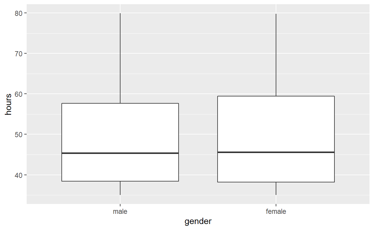
Females worked an average of 49.8 hours per week
Males worked an average of 49.6 hours per week
Use geom_boxplot to plot distributions of hours worked by gender
hr_2 %>%
  ggplot(aes(x = gender, y = hours)) +
  geom_boxplot()
specify the variables of interest are hours and gender
hr_2 %>%
  specify(response = hours, explanatory = gender)
Response: hours (numeric)
Explanatory: gender (factor)
# A tibble: 500 x 2
   hours gender
   <dbl> <fct>
 1  49.6 male
 2  39.2 female
 3  63.2 female
 4  42.2 male
 5  54.7 male
 6  54.3 female
 7  37.3 female
 8  45.6 female
 9  35.1 female
10  53   male
# ... with 490 more rows
hypothesize that the number of hours worked and gender are independent
hr_2  %>%
  specify(response = hours, explanatory = gender)  %>%
  hypothesise(null = "independence")
Response: hours (numeric)
Explanatory: gender (factor)
Null Hypothesis: independence
# A tibble: 500 x 2
   hours gender
   <dbl> <fct>
 1  49.6 male
 2  39.2 female
 3  63.2 female
 4  42.2 male
 5  54.7 male
 6  54.3 female
 7  37.3 female
 8  45.6 female
 9  35.1 female
10  53   male
# ... with 490 more rows
generate 1000 replicates representing the null hypothesis
hr_2 %>%
  specify(response = hours, explanatory = gender)  %>%
  hypothesize(null = "independence")  %>%
  generate(reps = 1000, type = "permute")
Response: hours (numeric)
Explanatory: gender (factor)
Null Hypothesis: independence
# A tibble: 500,000 x 3
# Groups:   replicate [1,000]
   hours gender replicate
   <dbl> <fct>      <int>
 1  55.2 male           1
 2  72.6 female         1
 3  59.1 female         1
 4  58.7 male           1
 5  66.8 male           1
 6  35.1 female         1
 7  50.6 female         1
 8  35.1 female         1
 9  49.2 female         1
10  35   male           1
# ... with 499,990 more rows
calculate the distribution of statistics from the generated data
Assign the output null_distribution_2_sample_permute
Display null_distribution_2_sample_permute
null_distribution_2_sample_permute  <- hr_2 %>%
  specify(response = hours, explanatory = gender)  %>%
  hypothesize(null = "independence")  %>%
  generate(reps = 1000, type = "permute")  %>%
  calculate(stat = "t", order = c("female", "male"))

null_distribution_2_sample_permute
# A tibble: 1,000 x 2
   replicate    stat
 *     <int>   <dbl>
 1         1  0.379
 2         2 -0.0940
 3         3 -0.943
 4         4  0.0654
 5         5 -0.0785
 6         6 -0.203
 7         7 -1.28
 8         8 -0.750
 9         9  0.467
10        10 -0.181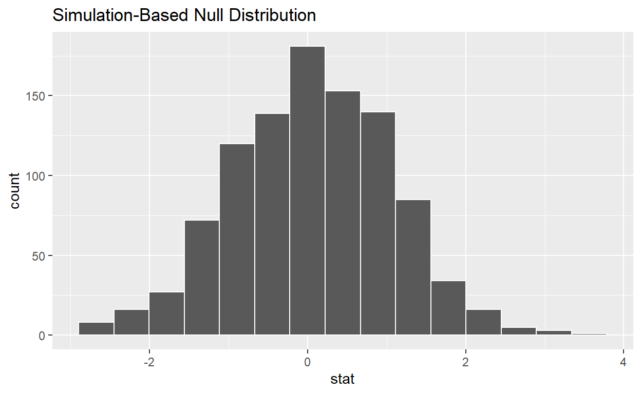
# ... with 990 more rowsvisualize(null_distribution_2_sample_permute)
calculate the stst from your observed data Assign the output observed_t_2_sample_stat
Display observed_t_2_sample_stat
observed_t_2__sample_stat  <- hr_2 %>%
  specify(response = hours, explanatory = gender)  %>%
  calculate(stat = "t", order = c("female", "male"))

observed_t_2__sample_stat
# A tibble: 1 x 1
   stat
  <dbl>
1 0.208
get_p_value from the simulated null distribution and the observed statistic
null_t_distribution  %>%
  get_p_value(obs_stat = observed_t_statistic, direction = "two-sided")
# A tibble: 1 x 1
  p_value
    <dbl>
1       0
shade_p_value on the simulated null distribution
null_t_distribution  %>%
  visualize() +
  shade_p_value(obs_stat = null_t_distribution, direction = "two-sided")

no, p-value is not less than .05
Does your analysis support the null hypothesis that the true mean number of hours worked by female and male employees was the same? yes
Question Anova
hr_anova <- read_csv("https://estanny.com/static/week13/data/hr_3_tidy.csv",
                col_types = "fddfff")
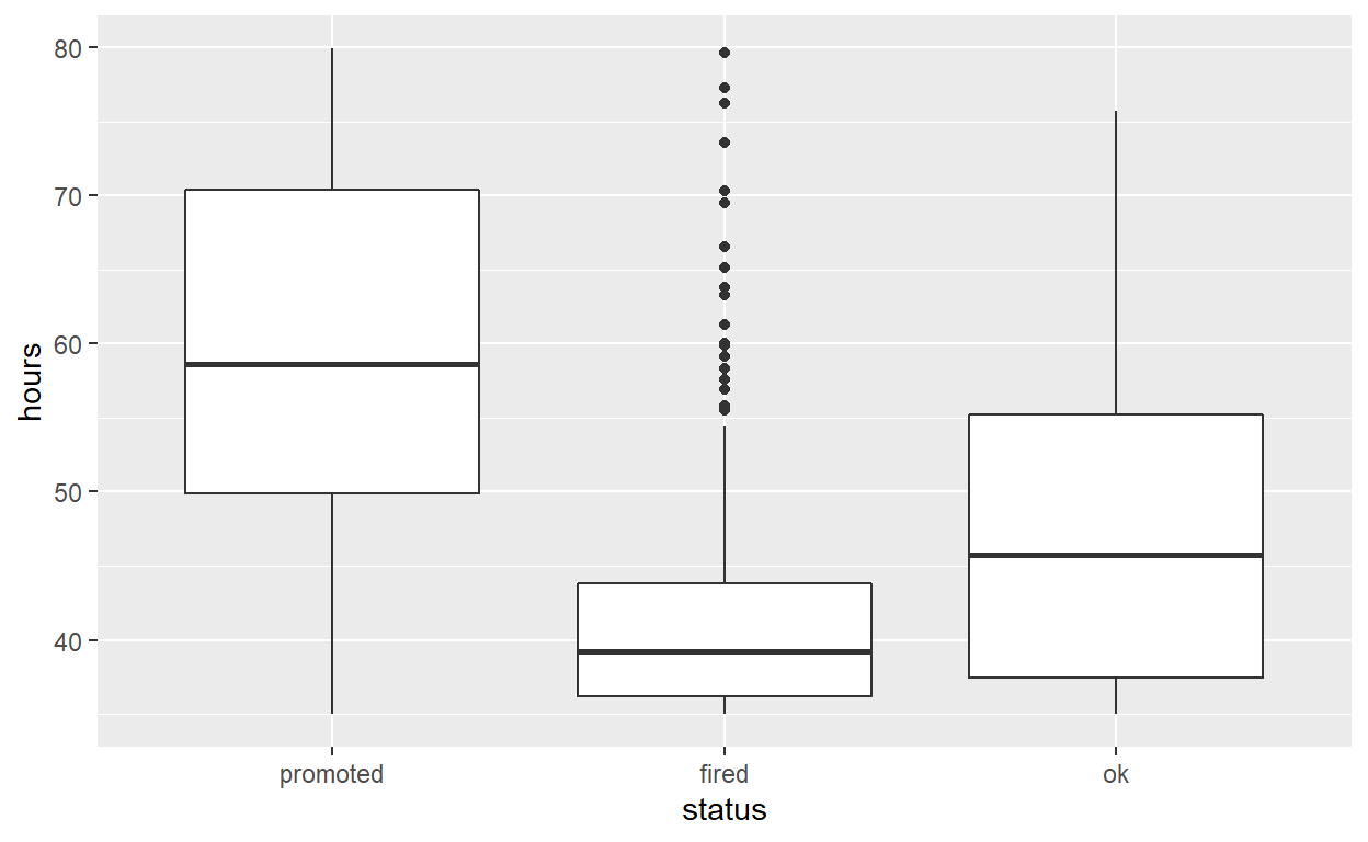
Q: Is the average number of hours worked the same for all three status (fired, ok and promoted) ? use skim to summarize the data in hr_anova by status
hr_anova %>%
  group_by(status)  %>%
  skim()
| Name | Piped data |
| Number of rows | 500 |
| Number of columns | 6 |
| _______________________ | |
| Column type frequency: | |
| factor | 3 |
| numeric | 2 |
| ________________________ | |
| Group variables | status |
Variable type: factor
| skim_variable | status | n_missing | complete_rate | ordered | n_unique | top_counts |
|---|---|---|---|---|---|---|
| gender | promoted | 0 | 1 | FALSE | 2 | fem: 91, mal: 81 |
| gender | fired | 0 | 1 | FALSE | 2 | mal: 98, fem: 98 |
| gender | ok | 0 | 1 | FALSE | 2 | mal: 68, fem: 64 |
| evaluation | promoted | 0 | 1 | FALSE | 4 | goo: 79, ver: 52, fai: 21, bad: 20 |
| evaluation | fired | 0 | 1 | FALSE | 4 | bad: 77, fai: 64, ver: 30, goo: 25 |
| evaluation | ok | 0 | 1 | FALSE | 4 | fai: 53, bad: 51, goo: 18, ver: 10 |
| salary | promoted | 0 | 1 | FALSE | 6 | lev: 42, lev: 37, lev: 36, lev: 28 |
| salary | fired | 0 | 1 | FALSE | 6 | lev: 59, lev: 40, lev: 39, lev: 25 |
| salary | ok | 0 | 1 | FALSE | 6 | lev: 33, lev: 29, lev: 28, lev: 23 |
Variable type: numeric
| skim_variable | status | n_missing | complete_rate | mean | sd | p0 | p25 | p50 | p75 | p100 | hist |
|---|---|---|---|---|---|---|---|---|---|---|---|
| age | promoted | 0 | 1 | 40.22 | 11.11 | 20.1 | 31.67 | 41.00 | 48.82 | 59.7 | ▆▇▇▇▇ |
| age | fired | 0 | 1 | 38.95 | 11.23 | 20.0 | 29.82 | 38.80 | 48.75 | 59.9 | ▇▆▇▇▅ |
| age | ok | 0 | 1 | 39.03 | 11.77 | 20.0 | 28.28 | 38.75 | 49.92 | 59.7 | ▇▇▆▇▆ |
| hours | promoted | 0 | 1 | 59.29 | 12.53 | 35.0 | 49.90 | 58.65 | 70.35 | 79.9 | ▅▆▇▆▇ |
| hours | fired | 0 | 1 | 42.37 | 9.15 | 35.0 | 36.20 | 39.20 | 43.80 | 79.6 | ▇▁▁▁▁ |
| hours | ok | 0 | 1 | 47.99 | 11.55 | 35.0 | 37.45 | 45.75 | 55.23 | 75.7 | ▇▃▃▂▂ |
hr_anova %>%
  ggplot(aes(x = status, y = hours)) +
  geom_boxplot()
specify the variables of interest are hours and status
hr_anova %>%
  specify(response = hours, explanatory = status)
Response: hours (numeric)
Explanatory: status (factor)
# A tibble: 500 x 2
   hours status
   <dbl> <fct>
 1  49.6 promoted
 2  39.2 fired
 3  63.2 promoted
 4  42.2 promoted
 5  54.7 promoted
 6  54.3 fired
 7  37.3 fired
 8  45.6 promoted
 9  35.1 fired
10  53   promoted
# ... with 490 more rows
hypothesize that the number of hours worked and status are independent
hr_anova  %>%
  specify(response = hours, explanatory = status)  %>%
  hypothesize(null = "independence")
Response: hours (numeric)
Explanatory: status (factor)
Null Hypothesis: independence
# A tibble: 500 x 2
   hours status
   <dbl> <fct>
 1  49.6 promoted
 2  39.2 fired
 3  63.2 promoted
 4  42.2 promoted
 5  54.7 promoted
 6  54.3 fired
 7  37.3 fired
 8  45.6 promoted
 9  35.1 fired
10  53   promoted
# ... with 490 more rows
generate 1000 replicates representing the null hypothesis
hr_anova %>%
  specify(response = hours, explanatory = status)  %>%
  hypothesize(null = "independence")  %>%
  generate(reps = 1000, type = "permute")
Response: hours (numeric)
Explanatory: status (factor)
Null Hypothesis: independence
# A tibble: 500,000 x 3
# Groups:   replicate [1,000]
   hours status   replicate
   <dbl> <fct>        <int>
 1  41.2 promoted         1
 2  36.5 fired            1
 3  35.1 promoted         1
 4  36.2 promoted         1
 5  35.1 promoted         1
 6  58.7 fired            1
 7  35.9 fired            1
 8  51.3 promoted         1
 9  42.3 fired            1
10  66.2 promoted         1
# ... with 499,990 more rows
calculate the distribution of statistics from the generated data
Assign the output null_distribution_anova
Display null_distribution_anova
null_distribution_anova  <- hr_anova %>%
  specify(response = hours, explanatory = gender)  %>%
  hypothesize(null = "independence")  %>%
  generate(reps = 1000, type = "permute")  %>%
  calculate(stat = "F")

null_distribution_anova
# A tibble: 1,000 x 2
replicate stat
* <int> <dbl>
1 1 6.58
2 2 0.150
3 3 0.203
4 4 0.0991
5 5 0.246
6 6 0.178
7 7 1.09
8 8 1.96
9 9 1.20
10 10 0.587
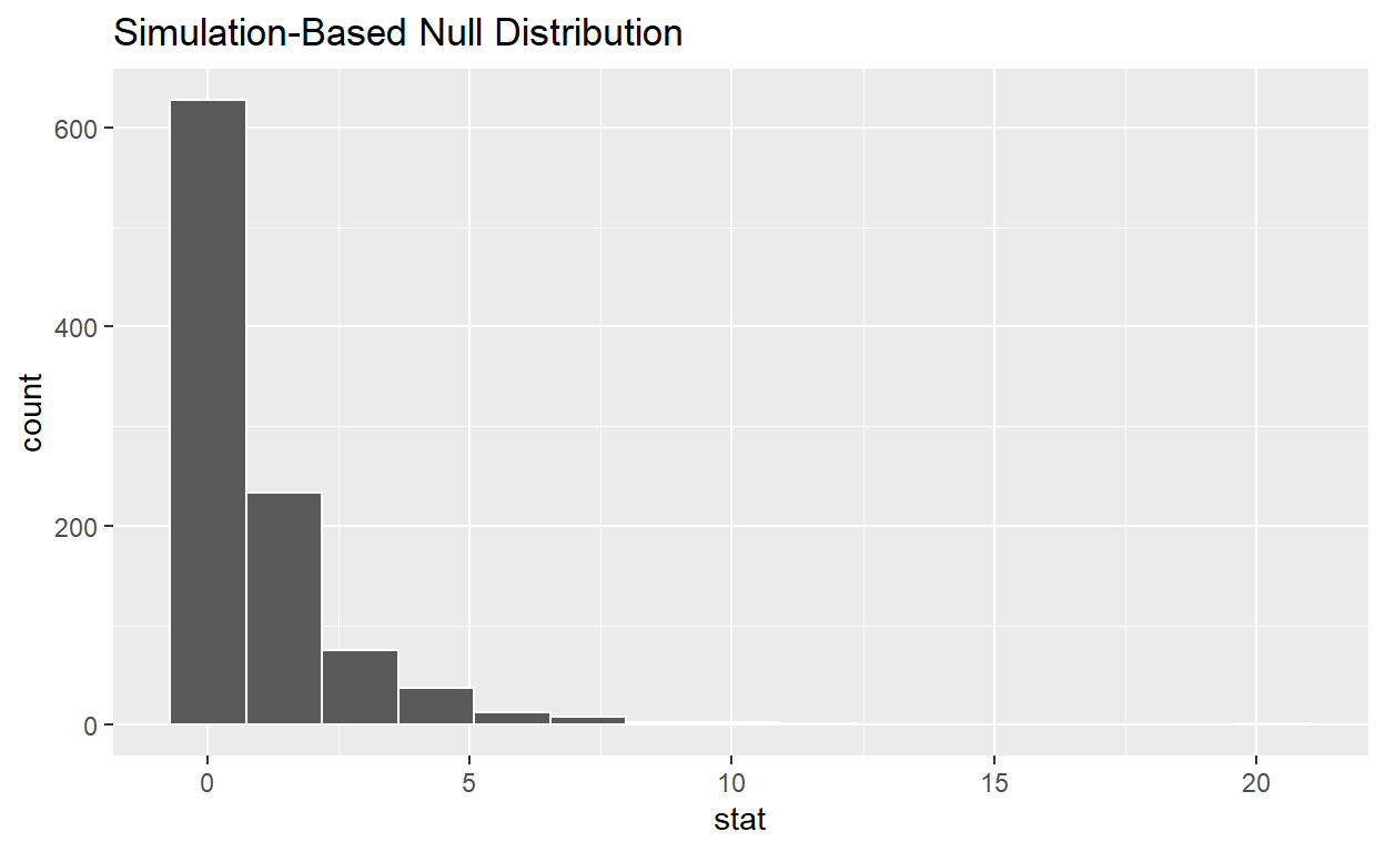
# ... with 990 more rowsvisualize the simulated null distribution
visualize(null_distribution_anova)
calculate the statistic from your observed data
Assign the output observed_f_sample_stat
Display observed_f_sample_stat
observed_f_sample_stat  <- hr_anova %>%
  specify(response = hours, explanatory = status)  %>%
  calculate(stat = "F")

observed_f_sample_stat
# A tibble: 1 x 1
   stat
  <dbl>
1  110.
get_p_value from the simulated null distribution and the observed statistic
null_distribution_anova  %>%
  get_p_value(obs_stat = null_distribution_anova , direction = "greater")
# A tibble: 1 x 1
  p_value
    <dbl>
1   0.291
shade p-value
null_distribution_anova  %>%
  visualize() +
  shade_p_value(obs_stat = null_distribution_anova, direction = "greater")
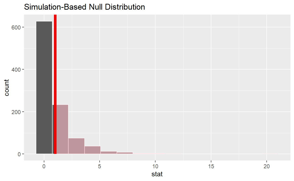
yes p-value less than .05
Does your analysis support the null hypothesis that the true means of the number of hours worked for those that were “fired”, “ok” and “promoted” were the same? no